Approximating Functions
Introduction
This fall semester I transferred from my community college in Kansas to the University of Colorado at Boulder to major in electrical engineering. One of my primary motivations for attending Boulder is the breadth of opportunities it offers in engineering, from clubs, classes, and research opportunities. So far I’ve not been disappointed respecting the latter, as at the start of the semester I had the good fortune to connect with Conor Rowan, a PhD candidate in the university’s Aerospace Department, who has generously agreed to mentor me in an area of his research related to using machine learning to find solutions to differential equations.
This last week we discussed how exactly you can approximate functions with a basis composed of other functions. Eventually, the plan is to learn about using optimization/machine learning techniques to find solutions to differential equations, and then apply this knowledge to a (hopefully) novel problem. All of this will surely inspire future articles, so stay tuned…
Motivation
To start, let us think about some ideas in terms of linear algebra and then generalize our findings into the continuous realm. Imagine that we have some vector $\textbf{v} \in \mathbb{R}^3$ and we would like to approximate this vector with the vectors $\textbf{v}_ \textbf{1} \in \mathbb{R}^3$ and $\textbf{v}_\textbf{2} \in \mathbb{R}^3$. Essentially, we’re trying to find the best approximation of $v$ by spanning two basis vectors.
$$ \bar{\textbf{v}} = \theta_1\textbf{v} _\textbf{1}+ \theta_2\textbf{v} _\textbf{2} $$
where $\theta_1$ and $\theta_2$ are parameters whose values we try to optimize for our approximation.
Now we want a way to measure the error between our approximation and $v$. A way to do this is simply subtract the two vectors
$$ \textbf{e}=\textbf{v}-\bar{\textbf{v}} $$
Furthermore, we can use this error vector to define a loss function
$$ L(\theta_1,\theta_2) = \frac{1}{2}\textbf{e} \cdot \textbf{e} $$
which is the squared length of the error vector $\textbf{e}$. When trying to find the best approximation, it’d be natural to try and minimize our loss function, which we can do by taking the gradient of the loss function with respect to each parameter and setting equal to zero. This will look like the following expressions:
$$ \frac{\partial L}{\partial \theta_1} = (\theta_1 \textbf{v} _\textbf{1} + \theta_2 \textbf{v} _\textbf{2} - \textbf{v})\textbf{v} _\textbf{1} = \textbf{e} \cdot \textbf{v} _\textbf{1} = 0 $$
$$ \frac{\partial L}{\partial \theta_2} = (\theta_1 \textbf{v} _\textbf{1} + \theta_2 \textbf{v} _\textbf{2} - \textbf{v})\textbf{f} _\textbf{2} = \textbf{e} \cdot \textbf{v} _\textbf{2} = 0 $$
The most important part of the these expressions to notice is that the dot product of the error vector and each of the basis vectors is 0, meaning the error has no component in the basis. Additionally, if we distribute the basis vectors that are outside of the parentheses in each of these equations and rearrange the term with $\textbf{v} \cdot \textbf{v} _\textbf{i}$ to the right side, hopefully it’s clear that we can represent these equations as the product of the matrix multiplication
$$ \begin{bmatrix} \textbf{v} _\textbf{1} \cdot \textbf{v} _\textbf{1} & \textbf{v} _\textbf{1} \cdot \textbf{v} _\textbf{2} \\ \textbf{v} _\textbf{2} \cdot \textbf{v} _\textbf{1} & \textbf{v} _\textbf{2} \cdot \textbf{v} _\textbf{2} \end{bmatrix} \begin{bmatrix} \theta_1 \\ \theta_2 \end{bmatrix} = \begin{bmatrix} \textbf{v} _\textbf{1} \\ \textbf{v} _\textbf{2} \end{bmatrix} $$
Crucially, we’ve created an equations of the form
$$ \textbf{K} \boldsymbol{\theta}=\textbf{F} $$
of which we can solve for $\boldsymbol{\theta}$ by multiplying each side by the inverse matrix of $\textbf{K}$, leaving us with the parameters that optimize our approximation!
Now we can move into approximating continuous functions, but now instead of our basis being composed of vectors it will be composed of functions:
$$ e(x) = v(x) - \sum_{i=1}^{N} \theta_i f_i(x) $$
where $e(x)$ is our error function, $v(x)$ is what we want to approximate, and each $f_i(x)$ is a function in our basis. We want to find the optimal parameters $\theta_i$, and to find them we proceed just as before, first defining a loss function
$$ L(\boldsymbol{\theta}) = \frac{1}{2}\int_{a}^{b} ((v(x) - \sum_{i=1}^{N} \theta_i f_i(x)) \ dx)^2 $$
Let’s find the gradient of the loss funtion with respect to each parameter. For $j=1,2,…,N$
$$ \frac{\partial L}{\partial \theta_j} = \int_{a}^{b} ((v(x) - \sum_{i=1}^{N} \theta_i f_i(x)) \frac{\partial}{\partial \theta_i} (v(x) - \sum_{i=1}^{N} \theta_i f_i(x))) \ dx $$
$$ = \int_{a}^{b} ((v(x) - \sum_{i=1}^{N} \theta_i f_i(x))v_j(x)) \ dx = 0 $$
We can see that our again that we’ve created a matrix of the same form above, where
$$ K_{ji} = \int_{a}^{b} f_j(x)f_i(x) \ dx $$
$$ F_j = \int_{a}^{b} v(x)f_j(x) \ dx $$
Here $j$ denotes the row of the matrix and $i$ the column. So after solving for the vector of parameters, we have know which parameters optimally approximate a function for a given basis. To see this idea in action I’ve made a demonstration in Colab which you can find here.
Computational Example
Let’s look at a simple implementation of the discussed method, where we’ll define a function we want to approximate, choose a collection of functions for our basis, and numerically perform the calculations.
In our first block of code we define the domain over which we’ll be evluating our functions and the number of samples we wish to take across the domain. Note that the larger your domain, the more samples you’ll want to take. Finally, we’ll define the function we wish to approximate and the basis functions.
domain = [0,10] # domain over which functions are evaluated
samples = 1000 # number of points at which functions evaluated at
f = '(np.exp(x) - x + np.sin(x))' # function we want to approximate
v = ['(x**2)','(x**3)','(1)'] # functions in approximation basis
N = len(v) # number of functions in basis
You’ll notice the perhaps strange looking syntax of storing our functions as strings. I’d never seen this syntax before, but I think it works really well for having fast and easy access to expressions without needing to repeatedly rewrite them or call them as functions. It works like this:
eq = "x + 3"
x = 3
result = eval(eq)
print(eq)
The print call will output 6 which is the obvious result of $x+3$. Basically, as long you’ve assigned a value to the variable in whose terms you wrote your equations, you can call eval() and it will plug in that value into the equation and return the result. Very cool! You’ll also want to wrap your expressions in parentheses so that we can multiply them today without any unintended consequences from the order of operations.
In the next code block we create our matrices that correspond to the matrices of the same names we’ve discussed above. What’s perhaps the most confusing part is the embedded loops, but hopefully you can draw the connection them and the way we “looped” through the indeces in the equations above. For additional clarity, I’ve been consistent in math and code with how I’ve labeled the indeces, so the $j$ index in the code corresponds to how the $j$ index is used in the math, and same for $i$. In essence, this block just calls an integration function on the proper functions and stores the results in the right matrix entry.
K = np.zeros((N,N)) # stiffness matrix
F = np.zeros((N,1)) # force matrix
for j in range(0,N):
  integrand = f + "*" + v[j]
  force = rectIntegration(integrand)
  F[j,0] = force

  for i in range(0,N):
    integrand = v[i] + "*" + v[j]
    stiff = rectIntegration(integrand)
    K[j,i] = stiff
Next up we’ll cover the rectIntegration() function. To help it make sense, here’s an image from Paul’s Online Math Notes (link).
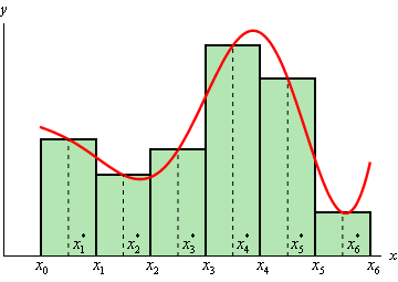
So in the code, we first find the spacing h between our samples, which corresponds to $x_i - x_{i-1}$ in the image. Next, we set the starting point to the first point in the domain plus h/2, so that we are in the middle of the first two samples. We also set up a list of points we’ll be iterating through so that we only evaluate our integrand at the midpoints of two sample points. Once we’re inside the loop, we evaluate the integrand (the height of the rectangle) and multiply it by h (the width of our rectangle), and we repeat this process so that we get an approximate area under the curve, which corresponds to the function’s integral.
# numerical integration function
def rectIntegration(integrand):
  h = (domain[1]-domain[0]) / samples # width of rectangles
  points = np.arange(domain[0]+h/2,domain[1],h) # evaluate middle point of rects
  result = 0 # store integration result
  for p in points:
    x = p
    result += (h * eval(integrand))

  return result
All that’s left to do is plot our results, and since that’s a nontechnical discussion I’ll leave us with this pretty graph:
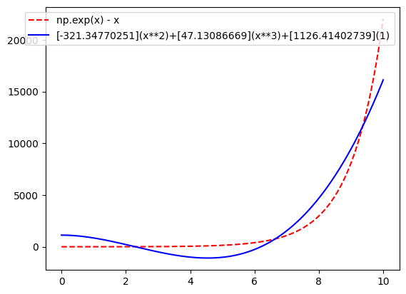
If you want to see the difference in how an approximation performs with a different amount of basis functions or different types of basis functions make sure you play around with the Colab code!