<?xml version="1.0" encoding="utf-8"?><feed xmlns="http://www.w3.org/2005/Atom" ><generator uri="https://jekyllrb.com/" version="4.4.1">Jekyll</generator><link href="https://finnlearns.fyi/feed.xml" rel="self" type="application/atom+xml" /><link href="https://finnlearns.fyi/" rel="alternate" type="text/html" /><updated>2026-08-05T22:22:02+00:00</updated><id>https://finnlearns.fyi/feed.xml</id><entry><title type="html">Simulating the Ising Model</title><link href="https://finnlearns.fyi/2025/11/02/ising.html" rel="alternate" type="text/html" title="Simulating the Ising Model" /><published>2025-11-02T00:00:00+00:00</published><updated>2025-11-02T00:00:00+00:00</updated><id>https://finnlearns.fyi/2025/11/02/ising</id><content type="html" xml:base="https://finnlearns.fyi/2025/11/02/ising.html"><![CDATA[<h3 id="introduction">Introduction</h3>
<p>As part of the probability class I’m taking, I have the option to create a poster to present at the end of the semester. Naturally, the topic must incorporate some aspect of probability, and as I researched it more I became fascinated with the applciations of probability to statistical mechanics. Topics in statistical mechanics also seem to lend themselves well to being simulated computationally, which is another area of interest. All in all, for my topic I ended up choosing one of the most common introductory examples of statistical physics: the Ising Model.</p>

<h3 id="physics">Physics</h3>
<p>The Ising Model attributes magnetism in a material to individual magnetic moments on a lattice, each of which can either be spin-up (+1) or spin-down (-1). We can model the overall energy of the material as</p>
<p style="latex-box">
$$ 
E = -\frac{J}{2} \sum_{i,j\in \Lambda} s_{i,j} (s_{i+1,j}+s_{i-1,j}+s_{i,j+1}+s_{i+1,j-1}) 
$$
</p>

<p>We will be working with square lattices only of length $L$, so in the energy formula $\Lambda=L^2$ is the “volume” of the lattice, and each $s_{i,j}$ is a magnetic moment at $i^{th}, j^{th}$ position. Additionally, $J$ is the interaction strength of the spins (which could be a different value for each pair of moments), but for simplicity’s sake we will set it to 1 for all pairs of moments. Furthermore, the energy formula technically has the extra term $\sum_{i}h_i s_i$, where $h_i$ represents a magnetic field at each moment. Again, for the sake of simplicity, we will set this term to zero for every moment. All in all, at the heart of the formula is the fact that the energy of the lattice is the sum of every moment mulitplied by the sum its nearest neighbours. The one-half term handles overcounting that occurs since this equation looks at all possible combinations, not just the unique ones that we care about.</p>

<p>A configuration of the lattice is an assignment of +1 or -1 to every moment of the lattice. Thus, for an $L$x$L$ lattice there are $2^{L^2}$ possible configurations. We represent a configuration as $c$ and the energy corresponding to $c$ as $E(c)$. We’re interested in observing phase transitions in the material using magnetization as an observable. This next part will feel like a lot of hand-waving (because there is on my part), but we can calculate an observable using the formula</p>
<p style="latex-box">
$$
\langle M \rangle = \frac{1}{Z(\beta)} \sum_{c}O(c)exp[-\beta E(c)]
$$
</p>
<p>$\beta = \frac{1}{k_B T}$, where $k_B$ is Boltzmann’s constant and $T$ is the temperature. Furthermore, in the preceding equation $Z(\beta) = \sum{c} exp[-\beta E(c)]$ is the canonical partition function. I myself am still figuring out why this equation is useful and how it is derived, but from what I understand it acts as a normalizing constant in the equation for the observable. The important aspect to note is that the equation for the observable sums across all possible configurations of the lattice, which we’ve already noted is $2^{L^2}$, a prohibitively large number for anything but the smallest of lattices. Therefore, we need a way to generate a smaller number of configurations that will give us a good approximation.</p>

<h3 id="simulation">Simulation</h3>
<p>Monte Carlo simulations is essentially just a name given to any algorithm that simulates a process via random sampling. Examples including modeling investment portfolio returns or the spread of disease. You can even approximate integrals using a Monte Carlo method:</p>
<p style="latex-box">
$$
\int_{A}f(x)dx \approx \frac{1}{N} \sum_{i=1}^{N} f(x_i)
$$
</p>

<p>First, we need to briefly describe what a Markov chain is: it’s basically a description of possible events in which the probability of the next event is only dependent on the current state. In other words, it is a memoryless process. In terms of simulating the Ising model, P(c \rightarrow c’) is the probability that we move from the current configuration $c$ to some configuration $c’$; note how it only depends on where we currently are in the process. If we do a memoryless random walk through the possible configurations, the Markov chain has the special property that the probability of being in configuration $c$ is \pi (c), the stationary distribution. Thus, we’ll construct a Markov chain with the stationary distribution $\pi(c) = exp(-\beta E(c))$.</p>

<p>The Metropolis-Hastings Algorithm provides a way to accomplish just this. It’s a three step process:</p>

<blockquote>
  <ol>
    <li>Start a configuration $c$</li>
    <li>Propose a move to a new configuration $c’$ with probability $P(c \rightarrow c’)$</li>
    <li>Accept the move to $c’$ with probability $\textbf{min}(1, \frac{\pi (c’)}{\pi (c)} \frac{P(c’ \rightarrow c)}{P(c \rightarrow c’)})$</li>
  </ol>
</blockquote>

<p>In the Metropolis-Hastings Algorithm we we propose moves that are equiprobable both ways, $P(c \rightarrow c’) = P(c’ \rightarrow c)$. We accomplish this by changing one single spin of the existing configuration. I also find it helpful to think about the probability of moving to the new configuration in terms of energy. Because the transition probabilities are the same they simply reduce to 1, and we’ve seen already that $\pi(c’) = exp(-\beta E(c’))$ and $\pi(c) = exp(-\beta E(c))$. Thus, $\frac{\pi (c’)}{\pi (c)} =\frac{exp(-\beta E(c’))}{exp(-\beta E(c))} = exp(-\beta \delta E)$. If $E(c’) &lt; E(c) \rightarrow exp(-\beta \delta E) &gt; 1$. What this tells us is that if the proposed configuration is of lower energy than the current configuration, we unconditioanlly move to it, which makes physical sense as systems always try to move into states of lower energy in the absence of energy sources. If $\frac{\pi (c’)}{\pi (c)} &lt; 0$ we accept the move with probability $exp(- \beta \delta E)$, so that we’re sampling from the probability distribution of our configurations.</p>

<p>Here, each $x_i$ is a uniformly distributed randomly chosen sample in the domain $A$, and as $N \rightarrow \infty$ the approximation converges to the actual solution. So the problem we’re trying to solve is how to best choose random configurations of the lattice that will give us a good approximation of the material’s behavior. Since each configuration of the lattice appears with probability $P(c) = exp(-\beta E(c))$ what we’d like to have is a way to generate configurations with such a probability.</p>

<h3 id="implementation">Implementation</h3>
<p>So what does it look like to computationally perform the Metropolis-Hastings algorithm? Well, I’ve written a mediocre C++ program to explore this question. Because the code is fairly complex (at least for me), the full code can be found <a href="https://github.com/FinnLearns/IsingModel/tree/main" title="Link to GitHub repository">here</a>, but I’ll just break down the interesting parts.</p>

<div class="language-cpp highlighter-rouge"><div class="highlight"><pre class="highlight"><code><span class="k">for</span> <span class="p">(</span><span class="kt">double</span> <span class="n">b</span> <span class="o">=</span> <span class="n">betaLower</span><span class="p">;</span> <span class="n">b</span> <span class="o">&lt;=</span> <span class="n">betaUpper</span><span class="p">;</span> <span class="n">b</span><span class="o">+=</span> <span class="n">betaStep</span><span class="p">)</span>
<span class="p">{</span>
    <span class="n">magnetArray</span> <span class="o">=</span> <span class="p">{};</span>
    <span class="n">myGen</span><span class="p">.</span><span class="n">setInitialConfig</span><span class="p">();</span>
        
    <span class="k">for</span><span class="p">(</span><span class="kt">size_t</span> <span class="n">n</span> <span class="o">=</span> <span class="mi">0</span><span class="p">;</span> <span class="n">n</span> <span class="o">&lt;</span> <span class="n">N</span><span class="p">;</span> <span class="o">++</span><span class="n">n</span><span class="p">)</span>
    <span class="p">{</span>
        <span class="n">magnet</span> <span class="o">=</span> <span class="n">myGen</span><span class="p">.</span><span class="n">getCurrMag</span><span class="p">();</span>
        <span class="n">magnetArray</span><span class="p">.</span><span class="n">push_back</span><span class="p">(</span><span class="n">magnet</span><span class="p">);</span>
        
        <span class="k">for</span> <span class="p">(</span><span class="kt">size_t</span> <span class="n">l</span> <span class="o">=</span> <span class="mi">0</span><span class="p">;</span> <span class="n">l</span> <span class="o">&lt;</span> <span class="n">volume</span><span class="p">;</span> <span class="o">++</span><span class="n">l</span><span class="p">)</span>
        <span class="p">{</span>
            <span class="n">rand1</span> <span class="o">=</span> <span class="n">engine</span><span class="p">()</span> <span class="o">%</span> <span class="n">volume</span><span class="p">;</span>
            <span class="n">rand2</span> <span class="o">=</span> <span class="k">static_cast</span><span class="o">&lt;</span><span class="kt">double</span><span class="o">&gt;</span><span class="p">(</span><span class="n">engine</span><span class="p">())</span> <span class="o">/</span> <span class="n">RAND_MAX</span><span class="p">;</span>
            <span class="n">myGen</span><span class="p">.</span><span class="n">updateLattice</span><span class="p">(</span><span class="n">b</span><span class="p">,</span> <span class="n">rand1</span><span class="p">,</span> <span class="n">rand2</span><span class="p">);</span>
        <span class="p">}</span>
    <span class="p">}</span>
<span class="p">}</span>
</code></pre></div></div>

<p>In this code we’re looping through a collection of $\beta$ values, effectively testing the lattice’s behavior at different temperatures. Before we begin sampling new configurations, we set our lattice to a cold start (every spin is either +1 or -1) using the line <code class="language-plaintext highlighter-rouge">myGen.setInitialConfig();</code> where <code class="language-plaintext highlighter-rouge">myGen</code> is an instance of the class <code class="language-plaintext highlighter-rouge">Ising</code> that contains methods for simulating and measuring the Ising model. We then enter the configuration loop, where for each $\beta$ value we sample 10,000 configurations, which is a number large enough for our generated configurations to be largely noncorrelated. At the beginning of each pass through the loop we also store the magnetization of the previous configuration:</p>
<p style="latex-box">
$$
    M(c) = \frac{1}{L^2} \sum_{i,j \in \Lambda} s_{i,j}
$$
</p>

<p>The method <code class="language-plaintext highlighter-rouge">updateLattice()</code> is then called:</p>
<pre><code class="language-cpp">void Ising::updateLattice(double currentBeta, int rand1, double rand2)
{
    int oppositeSpin = -1 * latticeSpin[rand1];
    
    int neighbourSum = latticeSpin[neighbourArray[rand1][0]] + latticeSpin[neighbourArray[rand1][1]]
                        + latticeSpin[neighbourArray[rand1][2]] + latticeSpin[neighbourArray[rand1][3]];
                        
    int deltaEnergy = latticeSpin[rand1] * neighbourSum * 2;

    if (exp(-1 * deltaEnergy * currentBeta) &gt; rand2)
    {
        latticeSpin[rand1] = oppositeSpin;
        currMag += 2 * oppositeSpin;
    }
}
</code></pre>

<p>We start by flipping a random spin of our lattice. We then need to calculate the energy difference between our current configuration and the proposed configuration. You could sum through all the magnetizations of both the original and proposed lattices and take their difference, but that would be extraordinarily time intensive. Instead, we remember that each new configuration changes the spin of only one moment, meaning the change is only local to that moment and its nearest neighbours. Thus we are able to derive the expression $\delta E = \frac{1}{2} s_{i,j} (s_{i+1,j} + s_{i-1,j} + s_{i,j+1} + s_{i,j-1})$, assuming the simplifications we made at the beginning. We then check if our acceptance conditions are met, and if it is we accept the move. Notice also that because the magnetization changes by only one spin we are able to keep a running tally of the magnetization of the material, instead of having to recompute the sum of the entire lattice every new configuration.</p>

<p>It’s also worth noting how the lattice is stored. Instead of creating an $LxL$ array, we can store it in a one-dimensional array by using a super-index, where every $i^{th}, j^{th}$ moment is stored at the $I = i + Lj$ index. The lattice also implements periodic boundary conditions, meaning moments at the edges are treated as neighbours to moments at opposite edge. To make accessing neighbours easier, we implement the array <code class="language-plaintext highlighter-rouge">neighbourArray</code>, which is of dimensions $L^2 x 4$. The row indeces correspond to the super-index we’re at on our lattice, and the four “column” indeces correspond to the superindeces of the four nearest neighbours. That’s implemented at the beginning of the algorithm with this method:</p>
<pre><code class="language-cpp">void Ising::findNeighbours()
{
    for (int superI = 0; superI &lt; L*L; superI++)
    {
        if (superI - 1 &gt;= 0) neighbourArray[superI][0] = superI - 1;
        else neighbourArray[superI][0] = superI + (L-1);
        
        if (superI + L &lt; L*L) neighbourArray[superI][1] = superI + L;
        else neighbourArray[superI][1] = superI - (L*(L-1));
        
        if (superI + 1 &lt; L*L) neighbourArray[superI][2] = superI + 1;
        else neighbourArray[superI][2] = superI - (L-1);
        
        if (superI - L &gt;= 0) neighbourArray[superI][3] = superI - L;
        else neighbourArray[superI][3] = superI + L*(L-1);
    }
}
</code></pre>

<p>Finally, after each pass through our configurations loop we output the magnetization of the lattice inside a file. Thus, for each $\beta$ value we will have a file with $N$ magnetizations corresponding to each of our $N$ proposed configurations.</p>

<h3 id="measurements-and-results">Measurements and Results</h3>
<p>An important preliminary to mention is that before we begin making measurements based on the magnetizations we recorded, we wait a certain number of steps so that our magnetization values settle around their equilibrium. If we don’t do this, our measurements will be off.</p>

<p>We are interested in taking four particular measurements of our model:</p>
<blockquote>
  <ol>
    <li>Mean magnetization: $m = \frac{1}{N} \sum_{n=1}^{N} M_n$ Basically we’re just taking the averages of the magnetizations produced by the Metropolis-Hastings algorithm at a certain temperature.</li>
    <li>Susceptibility: $\chi = \mu_2 V$. This is a measure of the variance amongst our magnetization values.</li>
    <li>Skewness: $B_3 = \frac{\mu_3}{(\mu_2)^\frac{3}{2}}$. At my level of understanding this measurement doesn’t mean much, but it essentially gives information about the symmetry of the distribution of the magnetizations.</li>
    <li>Kurtosis: $B_4 = \frac{\mu_4}{(\mu_2)^2}$. Again, at my level of understanding I’m not able to gain much insight out of this measurement yet. It was mostly included for thoroughness.</li>
  </ol>
</blockquote>

<p>In the measurement definitions each $\mu_k = \frac{1}{N} \sum_{n=1}^{N} (M_n - m)^k$ Measuring these in the code is fairly trivial, but what isn’t trivial is the results:</p>

<p align="center">  
    <img src="/assets/images/blog/ising/isingResults.png" width="50%" height="50%" />
</p>

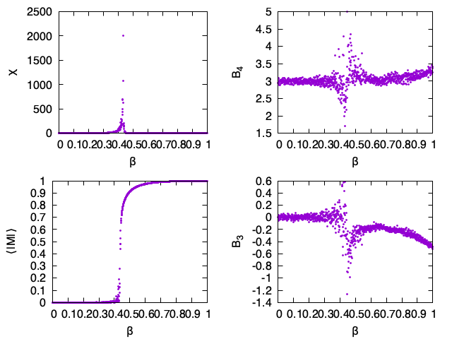
<p>We see that there is a sudden transition occuring in $m$ close to $\beta = 0.45$ and a discontinuity in $\chi$ at around the same point. Even in the skewness and kurtosis plots we can see irregular behavior at this point. From the definition of the mean. Basically what we’re is seeing is that for $\beta &lt; ~0.45$ there is a roughly equal number of moments that are spin-up and spin-down. However, as we pass through $\beta = ~0.45$ the spin-up moments become dominant, until they near instantaneously are the primary spin amongst the lattice. Remember that we start the lattice at each $\beta$ in a cold start, which in the case of this particular graph was a cold start at spin-up, or +1. Also remember that $\beta$ is inversely proportional to temperature. Thus, what we’re seeing is that at high temperatures the moments equally distributed between spin-up and spin-down, but as temperature decreases we hit a <em>phase transition</em> where the moments hardly change from where they were set in the cold start. This also makes physical sense: moments can’t just change spins randomly because that requires energy. So as the temperature decreases, representing less energy in the form of heat available to the lattice, the moments primarily stay in their initial states.</p>

<p>I’ve made a gif of the lattice’s simulated behavior around the phase transition. Notice how there are more spin-up moments on average. It’s also interesting to note how moments of a certain spin tend to coagulate around each other.</p>

<p align="center">  
    <img src="/assets/images/blog/ising/ising.gif" width="50%" height="50%" />
</p>

<h3 id="note-and-acknowledgement">Note and Acknowledgement</h3>
<p>I should note that in I’ve been implicitly using unitless quantities during this discussion, where our unitless variables are $\hat{\beta} = J \beta$ and $\hat{E} = \frac{E}{J}$. But as we simplified $J$ to $1$, this detail wasn’t especially important. Also, I should acknowledge some resources I used to help me with the implementation of the code and my own understanding of simulating the Ising model. First is an <a href="https://itp.uni-frankfurt.de/~mwagner/teaching/C_WS19/projects/Ising_proj.pdf" title="Link to assignment">assignment</a> from Goethe University in Frankfurt, Germany, and the other being a <a href="https://courses.physics.illinois.edu/phys498cmp/sp2022/Ising/IsingModel.html" title="Link to resource">online resource</a> for a computational physics class at the University of Illinois Urbana Champaign, each of which has been respectively linked.</p>]]></content><author><name></name></author><summary type="html"><![CDATA[Introduction As part of the probability class I’m taking, I have the option to create a poster to present at the end of the semester. Naturally, the topic must incorporate some aspect of probability, and as I researched it more I became fascinated with the applciations of probability to statistical mechanics. Topics in statistical mechanics also seem to lend themselves well to being simulated computationally, which is another area of interest. All in all, for my topic I ended up choosing one of the most common introductory examples of statistical physics: the Ising Model.]]></summary><media:thumbnail xmlns:media="http://search.yahoo.com/mrss/" url="https://finnlearns.fyi/assets/images/blog/ising/isingTitlePic.jpg" /><media:content medium="image" url="https://finnlearns.fyi/assets/images/blog/ising/isingTitlePic.jpg" xmlns:media="http://search.yahoo.com/mrss/" /></entry><entry><title type="html">Approx1</title><link href="https://finnlearns.fyi/2025/09/07/approx1.html" rel="alternate" type="text/html" title="Approx1" /><published>2025-09-07T00:00:00+00:00</published><updated>2025-09-07T00:00:00+00:00</updated><id>https://finnlearns.fyi/2025/09/07/approx1</id><content type="html" xml:base="https://finnlearns.fyi/2025/09/07/approx1.html"><![CDATA[<h3 id="introduction">Introduction</h3>

<p>This fall semester I transferred from my community college in Kansas to the University of Colorado at Boulder to major in electrical engineering. One of my primary motivations for attending Boulder is the breadth of opportunities it offers in engineering, from clubs, classes, and research opportunities. So far I’ve not been disappointed respecting the latter, as at the start of the semester I had the good fortune to connect with Conor Rowan, a PhD candidate in the university’s Aerospace Department, who has generously agreed to mentor me in an area of his research related to using machine learning to find solutions to differential equations.</p>

<p>This last week we discussed how exactly you can approximate functions with a basis composed of other functions. Eventually, the plan is to learn about using optimization/machine learning techniques to find solutions to differential equations, and then apply this knowledge to a (hopefully) novel problem. All of this will surely inspire future articles, so stay tuned…</p>

<h3 id="motivation">Motivation</h3>

<p>To start, let us think about some ideas in terms of linear algebra and then generalize our findings into the continuous realm. Imagine that we have some vector $\textbf{v} \in \mathbb{R}^3$ and we would like to approximate this vector with the vectors $\textbf{v}_ \textbf{1} \in \mathbb{R}^3$ and $\textbf{v}_\textbf{2} \in \mathbb{R}^3$. Essentially, we’re trying to find the best approximation of $v$ by spanning two basis vectors.</p>
<p style="latex-box">
$$
\bar{\textbf{v}} = \theta_1\textbf{v} _\textbf{1}+ \theta_2\textbf{v} _\textbf{2}
$$
</p>
<p>where $\theta_1$ and $\theta_2$ are parameters whose values we try to optimize for our approximation.</p>

<p>Now we want a way to measure the error between our approximation and $v$. A way to do this is simply subtract the two vectors</p>
<p style="latex-box">
$$
\textbf{e}=\textbf{v}-\bar{\textbf{v}}
$$
</p>
<p>Furthermore, we can use this error vector to define a loss function</p>
<p style="latex-box">
$$
L(\theta_1,\theta_2) = \frac{1}{2}\textbf{e} \cdot \textbf{e}
$$
</p>
<p>which is the squared length of the error vector $\textbf{e}$. When trying to find the best approximation, it’d be natural to try and minimize our loss function, which we can do by taking the gradient of the loss function with respect to each parameter and setting equal to zero. This will look like the following expressions:</p>
<p style="latex-box">
$$
\frac{\partial L}{\partial \theta_1} = (\theta_1 \textbf{v} _\textbf{1} + \theta_2 \textbf{v} _\textbf{2} - \textbf{v})\textbf{v} _\textbf{1} = \textbf{e} \cdot \textbf{v} _\textbf{1} = 0
$$
</p>
<p style="latex-box">
$$
\frac{\partial L}{\partial \theta_2} = (\theta_1 \textbf{v} _\textbf{1} + \theta_2 \textbf{v} _\textbf{2} - \textbf{v})\textbf{f} _\textbf{2} = \textbf{e} \cdot \textbf{v} _\textbf{2} = 0
$$
</p>

<p>The most important part of the these expressions to notice is that the dot product of the error vector and each of the basis vectors is 0, meaning the error has no component in the basis. Additionally, if we distribute the basis vectors that are outside of the parentheses in each of these equations and rearrange the term with $\textbf{v} \cdot \textbf{v} _\textbf{i}$ to the right side, hopefully it’s clear that we can represent these equations as the product of the matrix multiplication</p>
<p style="latex-box">
$$
\begin{bmatrix} \textbf{v} _\textbf{1} \cdot \textbf{v} _\textbf{1} &amp; \textbf{v} _\textbf{1} \cdot \textbf{v} _\textbf{2} \\ \textbf{v} _\textbf{2} \cdot \textbf{v} _\textbf{1} &amp; \textbf{v} _\textbf{2} \cdot \textbf{v} _\textbf{2} \end{bmatrix} \begin{bmatrix} \theta_1 \\ \theta_2 \end{bmatrix} = \begin{bmatrix} \textbf{v} _\textbf{1} \\ \textbf{v} _\textbf{2} \end{bmatrix}
$$
</p>

<p>Crucially, we’ve created an equations of the form</p>
<p style="latex-box">
$$
\textbf{K} \boldsymbol{\theta}=\textbf{F}
$$
</p>
<p>of which we can solve for $\boldsymbol{\theta}$ by multiplying each side by the inverse matrix of $\textbf{K}$, leaving us with the parameters that optimize our approximation!</p>

<p>Now we can move into approximating continuous functions, but now instead of our basis being composed of vectors it will be composed of functions:</p>
<p style="latex-box">
$$
e(x) = v(x) - \sum_{i=1}^{N} \theta_i f_i(x)
$$
</p>
<p>where $e(x)$ is our error function, $v(x)$ is what we want to approximate, and each $f_i(x)$ is a function in our basis. We want to find the optimal parameters $\theta_i$, and to find them we proceed just as before, first defining a loss function</p>
<p style="latex-box">
$$
L(\boldsymbol{\theta}) = \frac{1}{2}\int_{a}^{b} ((v(x) - \sum_{i=1}^{N} \theta_i f_i(x)) \ dx)^2
$$
</p>

<p>Let’s find the gradient of the loss funtion with respect to each parameter. For $j=1,2,…,N$</p>
<p style="latex-box">
$$
\frac{\partial L}{\partial \theta_j} = \int_{a}^{b} ((v(x) - \sum_{i=1}^{N} \theta_i f_i(x)) \frac{\partial}{\partial \theta_i} (v(x) - \sum_{i=1}^{N} \theta_i f_i(x))) \ dx
$$
</p>
<p style="latex-box">
$$
= \int_{a}^{b} ((v(x) - \sum_{i=1}^{N} \theta_i f_i(x))v_j(x)) \ dx = 0
$$
</p>

<p>We can see that our again that we’ve created a matrix of the same form above, where</p>
<p style="latex-box">
$$ 
K_{ji} = \int_{a}^{b} f_j(x)f_i(x) \ dx
$$
</p>
<p style="latex-box">
$$
F_j = \int_{a}^{b} v(x)f_j(x) \ dx
$$
</p>

<p>Here $j$ denotes the row of the matrix and $i$ the column. So after solving for the vector of parameters, we have know which parameters optimally approximate a function for a given basis. To see this idea in action I’ve made a demonstration in Colab which you can find <a href="https://colab.research.google.com/drive/14mJ0r-okoqYZZvAF2JUS2Mt3entey1Eu?usp=sharing" title="Link to Colab code">here</a>.</p>

<h3 id="computational-example">Computational Example</h3>
<p>Let’s look at a simple implementation of the discussed method, where we’ll define a function we want to approximate, choose a collection of functions for our basis, and numerically perform the calculations.</p>

<p>In our first block of code we define the domain over which we’ll be evluating our functions and the number of samples we wish to take across the domain. Note that the larger your domain, the more samples you’ll want to take. Finally, we’ll define the function we wish to approximate and the basis functions.</p>

<pre><code class="language-py">domain = [0,10] # domain over which functions are evaluated
samples = 1000 # number of points at which functions evaluated at
f = '(np.exp(x) - x + np.sin(x))' # function we want to approximate
v = ['(x**2)','(x**3)','(1)'] # functions in approximation basis
N = len(v) # number of functions in basis
</code></pre>

<p>You’ll notice the perhaps strange looking syntax of storing our functions as strings. I’d never seen this syntax before, but I think it works really well for having fast and easy access to expressions without needing to repeatedly rewrite them or call them as functions. It works like this:</p>
<pre><code class="language-py">eq = "x + 3"
x = 3
result = eval(eq)
print(eq)
</code></pre>
<p>The print call will output <code class="language-plaintext highlighter-rouge">6</code> which is the obvious result of $x+3$. Basically, as long you’ve assigned a value to the variable in whose terms you wrote your equations, you can call <code class="language-plaintext highlighter-rouge">eval()</code> and it will plug in that value into the equation and return the result. Very cool! You’ll also want to wrap your expressions in parentheses so that we can multiply them today without any unintended consequences from the order of operations.</p>

<p>In the next code block we create our matrices that correspond to the matrices of the same names we’ve discussed above. What’s perhaps the most confusing part is the embedded loops, but hopefully you can draw the connection them and the way we “looped” through the indeces in the equations above. For additional clarity, I’ve been consistent in math and code with how I’ve labeled the indeces, so the $j$ index in the code corresponds to how the $j$ index is used in the math, and same for $i$. In essence, this block just calls an integration function on the proper functions and stores the results in the right matrix entry.</p>
<pre><code class="language-py">K = np.zeros((N,N)) # stiffness matrix
F = np.zeros((N,1)) # force matrix
for j in range(0,N):
  integrand = f + "*" + v[j]
  force = rectIntegration(integrand)
  F[j,0] = force

  for i in range(0,N):
    integrand = v[i] + "*" + v[j]
    stiff = rectIntegration(integrand)
    K[j,i] = stiff
</code></pre>

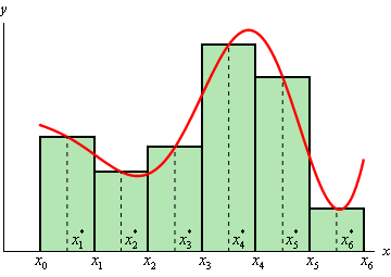
<p>Next up we’ll cover the <code class="language-plaintext highlighter-rouge">rectIntegration()</code> function. To help it make sense, here’s an image from Paul’s Online Math Notes (<a href="https://tutorial.math.lamar.edu/classes/calcii/ApproximatingDefIntegrals.aspx" title="Image source">link</a>).</p>

<p align="center">  
    <img src="/assets/images/blog/approx1Illustration.png" width="50%" height="50%" />
</p>

<p>So in the code, we first find the spacing <code class="language-plaintext highlighter-rouge">h</code> between our samples, which corresponds to $x_i - x_{i-1}$ in the image. Next, we set the starting point to the first point in the domain plus h/2, so that we are in the middle of the first two samples. We also set up a list of points we’ll be iterating through so that we only evaluate our integrand at the midpoints of two sample points. Once we’re inside the loop, we evaluate the integrand (the height of the rectangle) and multiply it by <code class="language-plaintext highlighter-rouge">h</code> (the width of our rectangle), and we repeat this process so that we get an approximate area under the curve, which corresponds to the function’s integral.</p>
<pre><code class="language-py"># numerical integration function
def rectIntegration(integrand):
  h = (domain[1]-domain[0]) / samples # width of rectangles
  points = np.arange(domain[0]+h/2,domain[1],h) # evaluate middle point of rects
  result = 0 # store integration result
  for p in points:
    x = p
    result += (h * eval(integrand))
    
  return result
</code></pre>

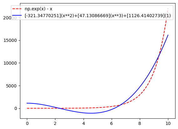
<p>All that’s left to do is plot our results, and since that’s a nontechnical discussion I’ll leave us with this pretty graph:</p>
<p align="center">  
    <img src="/assets/images/blog/approx1Title.png" width="50%" height="50%" />
</p>

<p>If you want to see the difference in how an approximation performs with a different amount of basis functions or different types of basis functions make sure you play around with the Colab code!</p>]]></content><author><name></name></author><summary type="html"><![CDATA[Introduction]]></summary><media:thumbnail xmlns:media="http://search.yahoo.com/mrss/" url="https://finnlearns.fyi/assets/images/blog/approx1Title.png" /><media:content medium="image" url="https://finnlearns.fyi/assets/images/blog/approx1Title.png" xmlns:media="http://search.yahoo.com/mrss/" /></entry><entry><title type="html">Website</title><link href="https://finnlearns.fyi/2025/07/12/website.html" rel="alternate" type="text/html" title="Website" /><published>2025-07-12T00:00:00+00:00</published><updated>2025-07-12T00:00:00+00:00</updated><id>https://finnlearns.fyi/2025/07/12/website</id><content type="html" xml:base="https://finnlearns.fyi/2025/07/12/website.html"><![CDATA[<h3 id="here-we-go-again">Here We Go Again</h3>

<p>July… the time of year when the temperatures rise, the flowers bloom, the children celebrate their freedom, and I bang my head against the computer trying to update my website. On the off chance that the dear reader has come across my previous website you might know that I updated it last year at around this same time. That website was built using the Django web framework, which turned out to be absolutely terrible for my purposes (i.e documenting my projects). Of course there’s a very high chance I was just using it wrong, but Django seems like it would be a lot more useful if you’re webiste has dynamic content or requires a database to keep track of large amounts of information, all of which my website neither has nor needs. Furthermore, the only way that I ever saw to actually write your own content was through the Django admin page, which requires a rich text editor plugin to be even remotely useable. Honestly, it wouldn’t be too hard to integrate one of those, but simply the fact that I had to persuaded me against using Django anymore for my website.</p>

<p>And so I searched far and wide for my website’s new digital home that would both be advanced enough for blogging yet simple enough that a web-design-infant such as I could use it. Enter: Jekyll. A static site generating machine that offers robust support for blogging applications in an intuitive system. If those people who’ve visited my last website are still reading they might still be wondering what the point of this entire project was since this site is literally a carbon-copy of the other aesthetically. But as they say, “beauty is only skin deep.” Because of Jekyll’s simplicity I was able to explore and include features that I otherwise wouldn’t have with Django, such as a code highlighter:</p>

<pre><code class="language-py"># a useless piece of python
def sum(x,y):
    sum = x + y
    return sum

num1 = 10
num2 = 20
mySum = sum(num1,num2)
print(mySum)
</code></pre>

<p>I can also use LaTeX for math expressions:</p>
<p style="latex-box">
$$
e^{(i\pi)} = cos(x) + isin(x)
$$
</p>

<p>Furthermore, Jekyll’s intuitiveness makes me much less daunted by the thought of adding new features, and I’ve already got a couple of future additions in mind. In particular, once I add some more projects to the site I’d like the ability to filter projects by certain attributes. I also want to add an interactive resume that summarizes my projects/education/experiences in a memorable and unique way (I’m not exactly sure what form this will take yet). In summary, keep checking back because I plan on updating this site much more regularly than my other one! And if you want a little more of a technical overview for the site, read on…</p>

<h3 id="jekyll">Jekyll</h3>

<p>Jekyll is static site generator that is based on the Ruby programming language, although proficiency with Ruby is not at all required to make a website with Jekyll; all you need is it installed on your computer. Before I continue, an important distinction should be made between dynamic and static websites: a static website’s content is simply premade html served by the web server and is not influenced by user input, while on the other hand the pages of a dynamic site are dynamically generated based on content in a database. That’s a gross oversimplification, but it highlights what I like about static sites: they require no backend and they’re easy to update.
Probably the most important part of Jekyll is the frontmatter on all your pages: this is data in the YAML format that is unique to each page and can be customized in virtually any way you want. Here’s a look at the first part of this very article you’re reading, where the frontmatter is inside the triple dashes:</p>

<pre><code class="language-css&gt;">---
layout: post
name: A Project Website
image: assets/images/blog/jekyll.png
type: project
keywords: website, jekyll, static website, FinnLearns, portfolio, personal website, project, web design
---

### Here We Go Again

July... the time of year when the temperatures rise, the flowers bloom, the children celebrate their freedom, ...
</code></pre>

<p>As you can see, there is data for the name, an associated image (the one you see in the project card), and keywords that will hopefully help with the visibility of my posts. There’s also the <code class="language-plaintext highlighter-rouge">type</code> frontmatter, which distinguishes between posts meant to be displayed in the Projects page or in the Life page. Finally, the layout frontmatter tells Jekyll which layout to apply to this page. Layouts in Jekyll are essentially CSS templates that wrap around the content of the site. Furthermore, layouts can inherit from other layouts, and in my case the post layout inherits from the default layout. The latter includes the CSS and styling for the navbar, the site colors, and all the CDN links needed for the code highlighter, styling, and LaTeX.</p>

<p>Speaking of the code highlighter, I am using <a href="https://prismjs.com">Prism</a> for that purpose, and it is being served through a CDN link. If you would like to do the same, I recommend just browsing the main page of its website which contains practically everything you need to start using it. For LaTeX I am using MathJax, which is a JavaScript library for formatting math expressions. Setting it up was extremely easy, mostly thanks to <a href="http://emily-hk.com/latex/">this</a> informative blog post. I’m also using the Bootstrap library for a couple of features throughout the site, most notably the cards in the Projects and Life pages. Also, utilizing static content in Jekyll is an absolute breeze compared to Django: inside a folder named “assets” you place your static content in appropriately titled subfolders for CSS, images, and JavaScript. And then when you want to access these resources you simply pass in the file path. Finally, to host the site I’m using Netlify, which is barely an inconvenience to setup as long as you follow their <a href="https://www.netlify.com/blog/2020/04/02/a-step-by-step-guide-jekyll-4.0-on-netlify/">instructions</a>. I’m not too familiar with it yet, so as of now I can’t offer any opinions that go beyond the setup process.</p>

<h3 id="in-conclusion">In Conclusion</h3>

<p>So there you have it! A (kind of) new website brimming with potential. Visitors of my previous site were undoubtedly dissapointed by the pace of my output (only six posts in a year), but I have ideas for some intersting projects in addition to more updates that I’d like to apply to the website, so check back often.</p>]]></content><author><name></name></author><summary type="html"><![CDATA[Here We Go Again]]></summary><media:thumbnail xmlns:media="http://search.yahoo.com/mrss/" url="https://finnlearns.fyi/assets/images/blog/jekyll.png" /><media:content medium="image" url="https://finnlearns.fyi/assets/images/blog/jekyll.png" xmlns:media="http://search.yahoo.com/mrss/" /></entry></feed>